Voronoi Diagrams From First Principles

Put four clinics on a city map and impose one rule: every address is served by the clinic closest to it. The rule is local. It only talks about one address at a time. Applied everywhere, it forces the whole map to break into territories.

The Local Rule

Start with two clinics, p and q. The addresses tied between them are exactly the points x where the distance to p equals the distance to q.

||x - p|| = ||x - q||

Squaring both sides removes the square roots. After expansion, the x.x terms cancel. What remains is linear in x, so the tie set is a line: the perpendicular bisector of the segment from p to q. One side belongs to p; the other belongs to q.

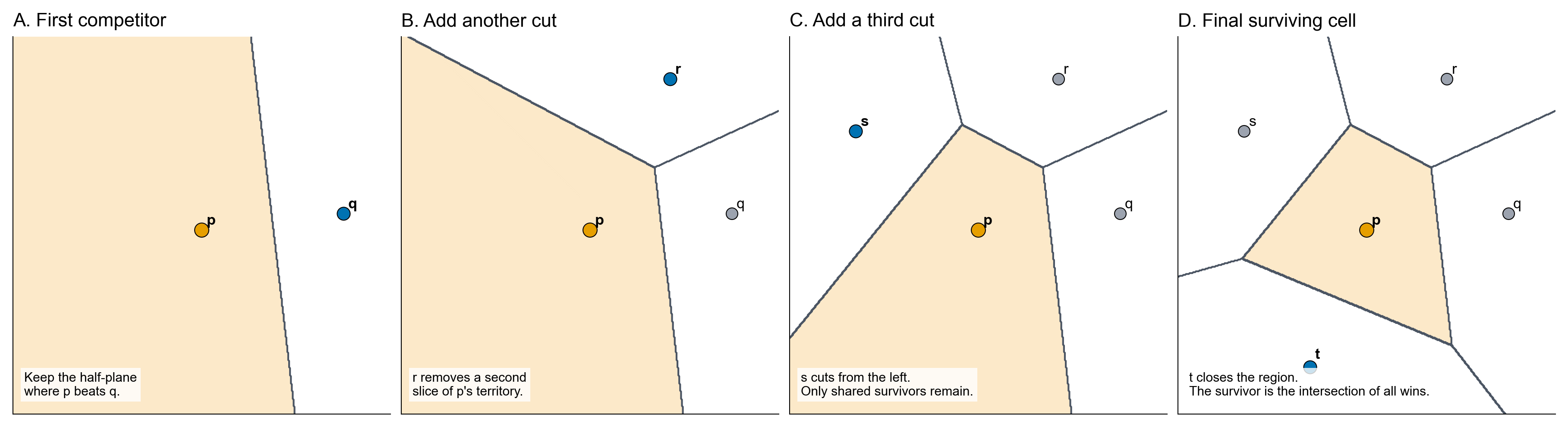
Interactive Figure 1. Nearest-Site Probe Move the sample point and switch focus sites to see how the nearest-site rule assigns territory.

Four panels show the territory of site p shrinking as competitors q, r, s, and t add half-plane cuts until the final Voronoi cell remains. — **Figure 1. Cell Carving Sequence** A Voronoi cell is the intersection of every half-plane where its site beats one competitor.

Cells Are Intersections

Adding a third clinic does not change the rule. It adds another contest. The region for p must lie on the p-side of the bisector between p and q, and also on the p-side of the bisector between p and r. Every new site contributes one more half-plane.

V(p_i) = {x : ||x - p_i|| <= ||x - p_j|| for every j != i}

That expression is the whole cell. A half-plane is convex, and an intersection of convex sets stays convex. A Voronoi cell can be unbounded, but it cannot have a dent. The boundary may run forever for a site on the outside of the point set; it still remains a convex polygonal chain.

Local Neighbors

Stand at a point where three cells meet. If the tied sites are p, q, and r, then the point is equally far from all three sites.

||x - p|| = ||x - q|| = ||x - r||

So there is a circle centered at x passing through p, q, and r. No other site can sit inside that circle. If one did, it would be closer to x than the three tied sites, and the three-way boundary point would disappear.

Connect two sites whenever their Voronoi cells share an edge. The resulting graph is the Delaunay graph. The Voronoi diagram organizes territory; the Delaunay graph records which sites are genuine local competitors.

Interactive Figure 2. Empty Circle and Delaunay Neighbors Switch the focus site or empty circle to see which shared Voronoi borders become Delaunay neighbor edges.

Sparse Structure

The definition talks about every pair of sites, but the final diagram keeps only local rivalries. In a generic planar input with n sites and h sites on the convex hull, the Delaunay triangulation has 3n - 3 - h edges and 2n - 2 - h triangles.

Duality transfers those counts back to the Voronoi diagram. Voronoi edges correspond to Delaunay edges, and Voronoi vertices correspond to Delaunay triangles. Since h >= 3, the planar Voronoi diagram has at most 3n - 6 edges and 2n - 5 vertices. The all-pairs rule collapses to a linear-size structure.

Computing the Whole Diagram

A direct cell-by-cell implementation is tempting: intersect the half-planes for one site, then repeat for every site. The mathematics is correct, but the computation is organized around polygons that are not independent. A shared edge or vertex can be rounded differently by neighboring cells, so locally plausible pieces may fail to glue into one diagram.

The standard algorithms keep the shared structure shared. Fortune’s algorithm sweeps a line across the sites and updates a beach line of parabolic arcs. The combinatorics change only at site events, where a new arc appears, and circle events, where a disappearing arc creates a Voronoi vertex.

The Delaunay-side view does the same repair through local adjacency. Insert a new site into the current triangulation, mark nearby edges as suspect, and apply one empty-circle test. Edges that pass are kept; edges that fail are flipped. Once the triangulation is locally Delaunay everywhere, the Voronoi diagram is its dual.

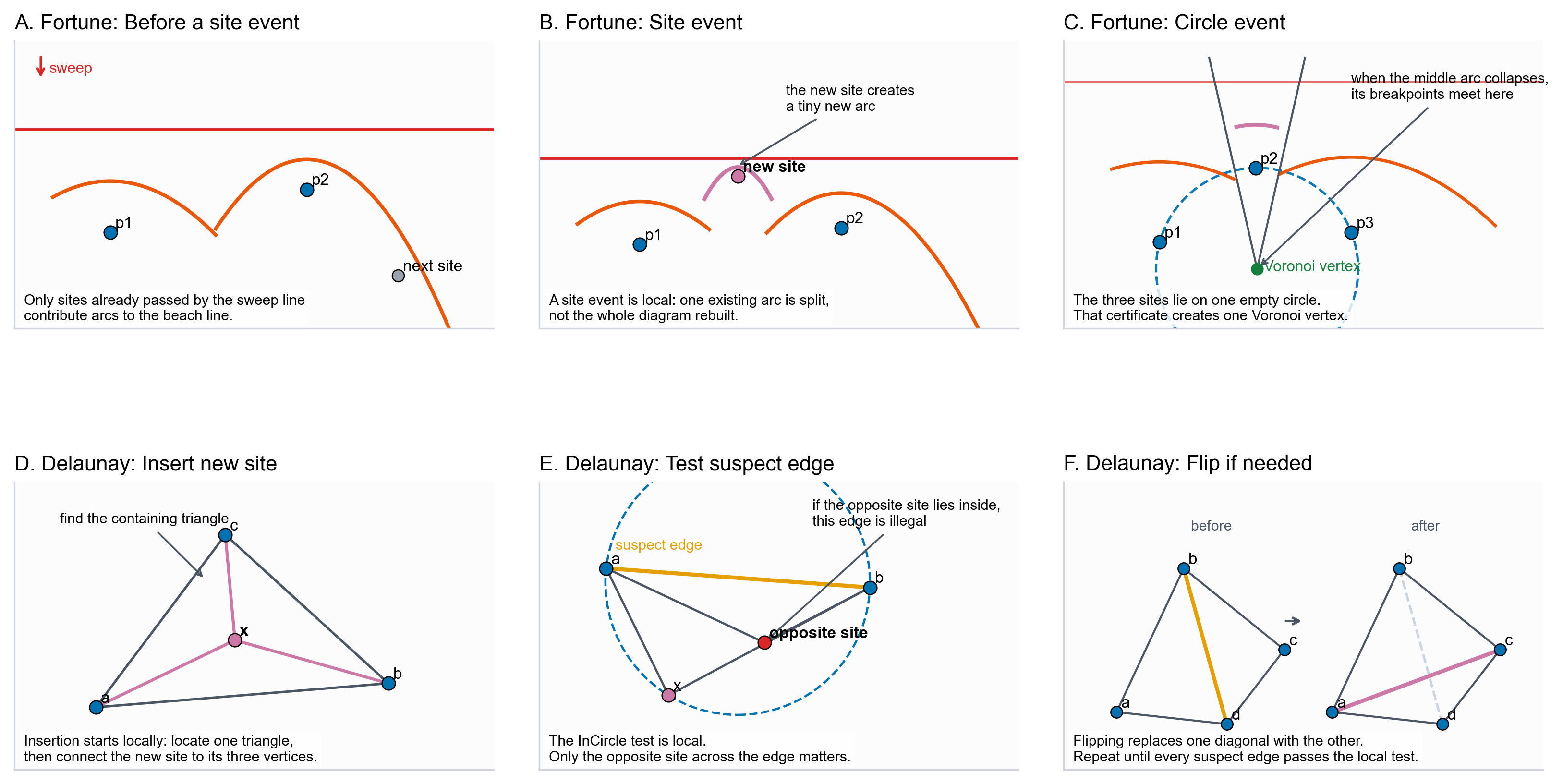
Six panels compare Fortune sweep-line events with Delaunay insertion, suspect-edge testing, and local edge flips. — **Figure 3. Algorithm Walkthroughs** Fortune's sweep line updates the beach line at events; Delaunay insertion repairs only local edges that fail the empty-circle test.

Lifting the Problem

Squared distance can be read as height above the plane. For one site s, the function D_s(x) = ||x - s||^2 is a paraboloid over the query point x. For many sites, the nearest site is the one whose paraboloid is lowest at that same x.

D_s(x) = ||x||^2 - 2x.s + ||s||^2

The term ||x||^2 is shared by every site, so it cannot change the winner at a fixed query point. Removing it leaves P_s(x) = -2x.s + ||s||^2, a plane. The lower envelope of distance paraboloids becomes the lower envelope of planes.

The Delaunay construction uses the same lift on the sites. Send each site to lambda(s) = (s, ||s||^2), take the convex hull, keep the lower faces, and project those faces back down. Three sites form a Delaunay triangle exactly when their lifted points share one lower supporting plane; its intersection with the paraboloid projects to the empty circumcircle through those sites.

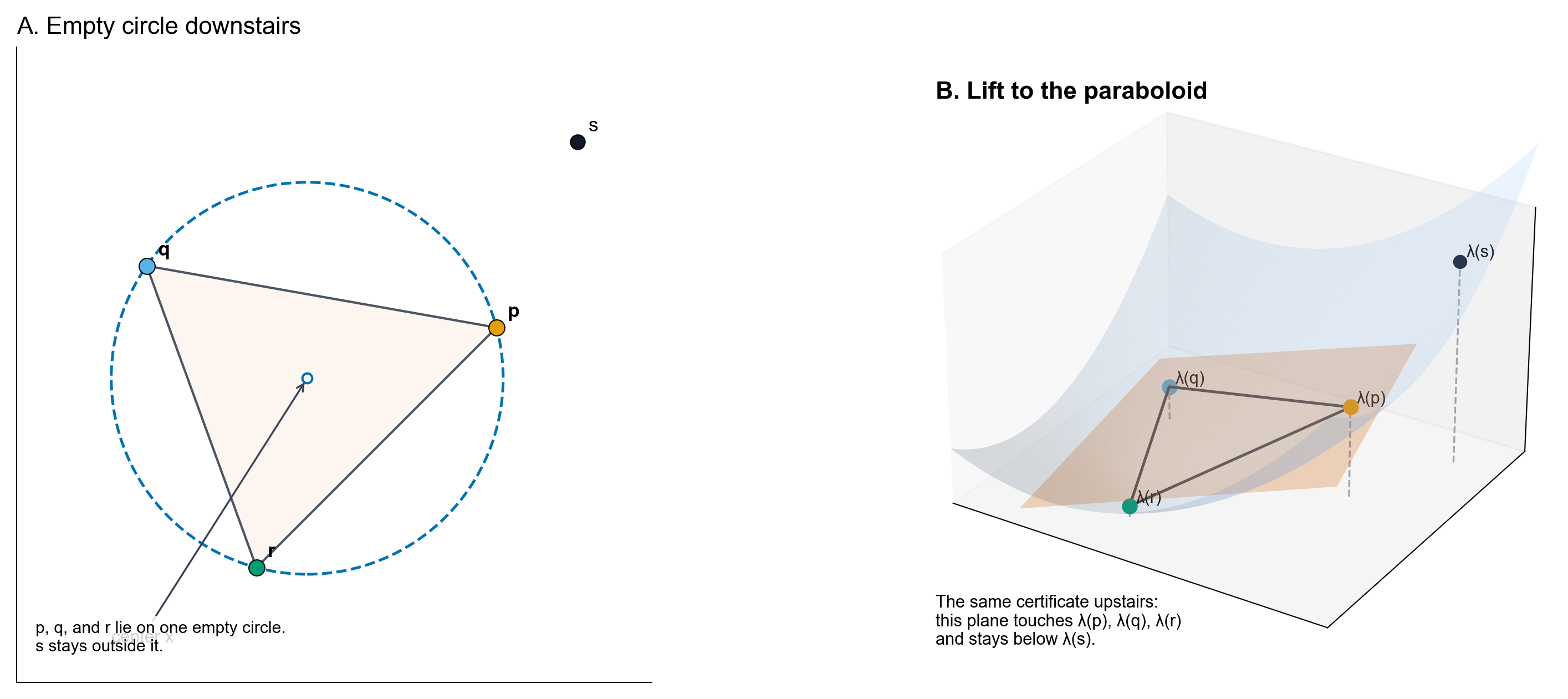
Two panels connect an empty circle through sites p, q, and r with a supporting plane through their lifted points on a paraboloid. — **Figure 4. Lifting Certificate** The empty circumcircle in the plane and the lower supporting plane upstairs are the same Delaunay certificate.

From Maps to Tokens

Keep the rule and change what the points mean. On a map, a point is an address and a site is a clinic. At a language-model output head, the point is the current hidden state h_t, and the sites are derived from token output weights.

For a token v, the final logit is z_v = h_t . w_v + b_v. Define c_v = w_v / 2 and beta_v = b_v + ||w_v||^2 / 4. Completing the square gives

h_t . w_v + b_v = -||h_t - c_v||^2 + beta_v + ||h_t||^2

The last term is the same for every token at that step, so it cannot change the winner. The readout is a power diagram: a weighted Voronoi partition of hidden-state space, one cell per token. This does not make the whole transformer a Voronoi diagram. It only describes the final linear contest that chooses the next token.

This view separates uncertainty from control. In free-text decoding, every token competes and some cell wins even near a boundary. If a controller masks answer tokens and leaves actions like ask, tool, or end, it does not enlarge an old abstain cell. It deletes inadmissible sites and redraws the smaller contest.

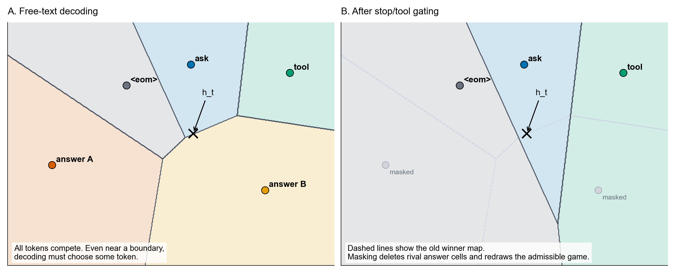
Two panels show free-text token winner regions around hidden state h_t and a redrawn partition after answer tokens are masked. — **Figure 5. Token Winner Regions** At the output head, token logits carve hidden-state space into weighted Voronoi cells; masking answer tokens redraws the admissible partition.

Structured Decoding Redraws the Menu

The redraw does not require new model weights. At each step, the model still scores the whole vocabulary. A decoder keeps a controller state s_t: where the grammar, parser, or tool schema says generation currently is.

From that state, the decoder computes the admissible token set A(s_t). It keeps logits for tokens inside that set, sets every other logit to -infinity, samples from the masked distribution, emits one token, updates the state, and repeats.

A fixed Boolean output is the smallest example. If the legal menu is only true and false, almost the whole vocabulary is crossed out and probability is renormalized over those 2 survivors. A tool call is stricter because the legal menu changes after each prefix: tool name, opening brace, field name, value, comma, or closing brace.

For scheduling, a schema can name missing slots such as person and timezone. If the controller exposes an ask_user action while ordinary answer prose is illegal, a clarifying question becomes an admissible continuation. This solves a format and action-availability problem. It does not automatically discover the deeper fact the user failed to state.

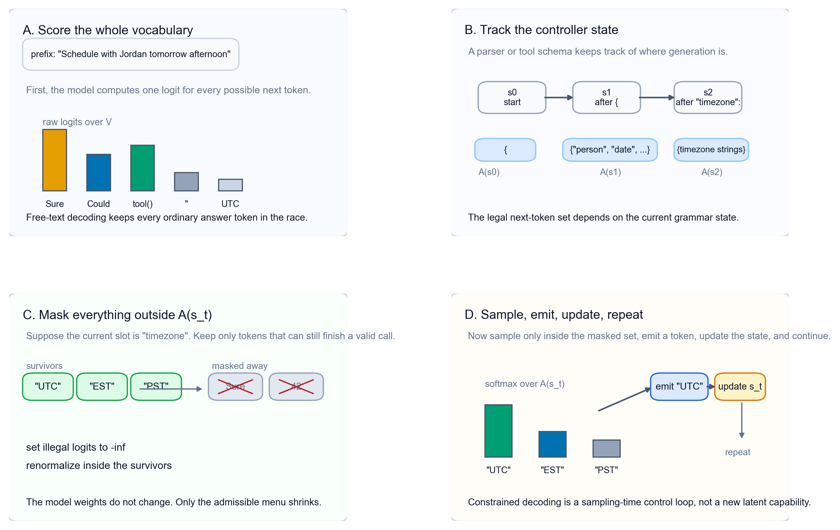
Four panels show a model scoring the whole vocabulary, a controller tracking parser state, illegal tokens masked away, and sampling repeated from the surviving set. — **Figure 6. Constrained Decoding Loop** A grammar or tool schema masks invalid next tokens, renormalizes over the survivors, and repeats after each emitted token.

Agentic Decoding Exposes Missing Slots

The scheduling example becomes sharper when the decoder is attached to tools. Free text asks the model to choose among answer-openers, question-openers, and stop tokens in one large contest. A tool loop can replace that contest with a smaller state machine: decide whether enough information exists, enter a JSON-like call, fill named fields, or ask for a missing value.

That is why shallow functional questions improve. If schedule_event requires person and timezone, those absences become explicit slots. The legal next actions can shrink to questions such as “Which Jordan?” or “Which timezone?” plus a few structural tokens.

This is still not a full theory of curiosity. The schema can expose fields it names, but it cannot discover every latent variable the user failed to state. Tool use solves format validity and action availability. Targeted clarification still needs an objective for choosing which uncertainty is worth reducing.

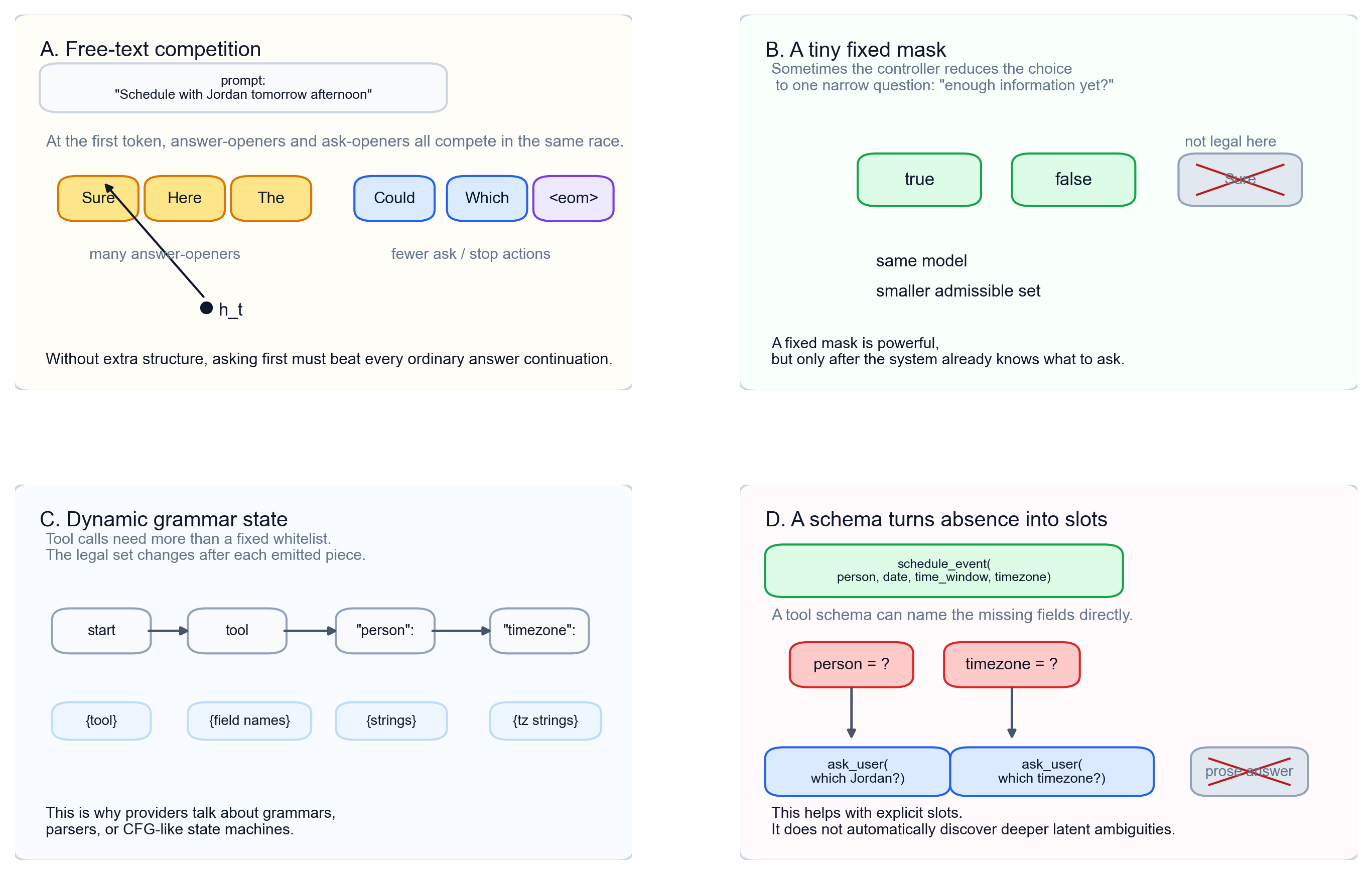
Four panels compare free-text token competition, a fixed Boolean mask, dynamic JSON grammar states, and tool calling with missing person and timezone slots. — **Figure 7. Agentic Decoding Story** Structured tool use turns a vague missing fact into named slots, grammar states, and a smaller set of legal next actions.

Source Boundary

The exact part of the story is local. Nearest-site cells, Delaunay duality, lifting, and power diagrams are standard geometry. The token-region derivation is algebra at the final linear output head. It is not a claim that every transformer layer is a Voronoi diagram.

The structured-decoding part is a decoder claim. A grammar or tool controller restricts the admissible next-token set; the model still scores the whole vocabulary. That gives format control and action availability. It does not give calibration or a general policy for deciding what information is missing.

The interpretation is narrower: targeted questioning needs an action space and objective that make asking a real move. If the question matters, the protocol has to name the missing slot, expose an ask or abstain action, or train and evaluate for information seeking. Next-token continuation alone does not reliably turn uncertainty into the right question.